Usage

Math Function Construction and Plotting

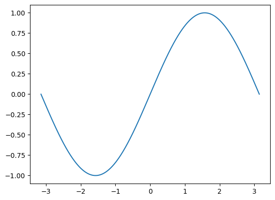
In GFuncPy, math functions are GridFunction objects that store \(x\) and \(y\) values. The most common way to create one is with Identity, which represents \(y = x\) on a grid. You can perform math operations and apply any NumPy univariate function (like sin, cos, exp, log, etc.) directly to these objects. See below examples.

\(\sin(x)\)

from gfuncpy import Identity, sin
from math import pi

x = Identity([-pi, pi])

sin(x).plot()

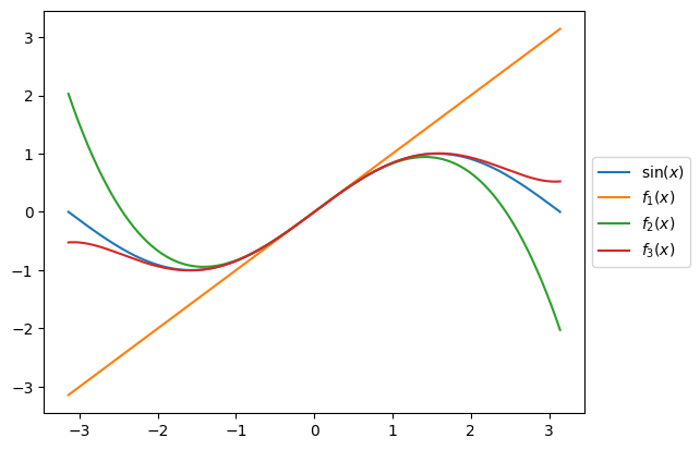
Taylor Series Approximations of \(\sin(x)\)

\[\sin(x) = x - \frac{x^3}{3!} + \frac{x^5}{5!} - \frac{x^7}{7!} + \dots.\]

sin(x).plot(label=r'$\sin(x)$')

f1 = x
f2 = x - x**3/6
f3 = x - x**3/6 + x**5/120

f1.plot(label='$f_1(x)$')
f2.plot(label='$f_2(x)$')
f3.plot(label='$f_3(x)$')

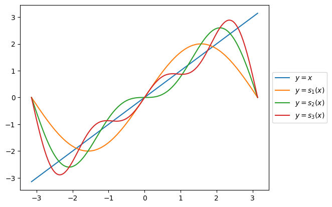
Fourier Series Approximations of \(y = x\)

In \(x\in (-\pi, \pi)\), the Fourier series of \(y = x\) is

\[x = 2\left(\sin(x) - \frac{\sin(2x)}{2} + \frac{\sin(3x)}{3} - \frac{\sin(4x)}{4} + \cdots\right).\]

x.plot(label=r'$y = x$')

s1 = 2*sin(x)
s2 = 2*(sin(x) - sin(2*x)/2)
s3 = 2*(sin(x) - sin(2*x)/2 + sin(3*x)/3)

s1.plot(label=r'$y=s_1(x)$')
s2.plot(label=r'$y=s_2(x)$')
s3.plot(label=r'$y=s_3(x)$')

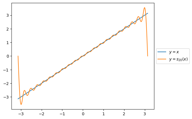
def s(n):
    return 2 * sum((-1)**(k+1) * sin(k*x)/k for k in range(1, n+1))

x.plot(label=r'$y=x$')
s(20).plot(label=r'$y=s_{20}(x)$')

Numerical Computations

Root Finding

Root of \(x^2 - 2\) in the range \(x\in[0, 2]\) is \(\sqrt 2\).

from gfuncpy import Identity, arctan

x = Identity([0, 2])

(x**2 - 2).root()

1.414212389380531

Point Value of a Function

Example:

\[4\arctan(1) = \pi.\]

f = arctan(x)

4*f(1)

3.141592653589793

Definite Integral

Example:

\[\int_0^1 \frac{4}{x^2 + 1}\,dx = \pi.\]

(4/(x**2 + 1)).integrate(frm=0, to=1)

3.141588486923126

Indefinite Integral

Example:

\[\int_{-\pi}^x \cos(u)\,du = \sin(x).\]

from gfuncpy import Identity, sin, cos
from math import pi

x = Identity([-pi, pi])


cos(x).integrate().plot(label=r'$\int\cos(x)\,dx$')

sin(x).plot(label=r'$\sin(x)$')

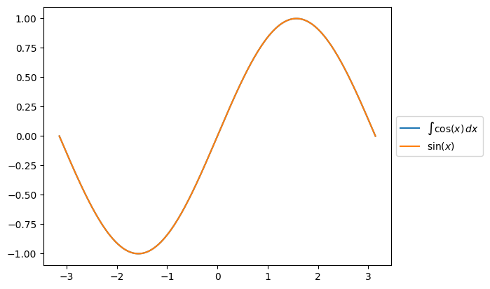
You can also use the alias int for integrate, e.g. cos(x).int().plot().

More on Math Function Construction

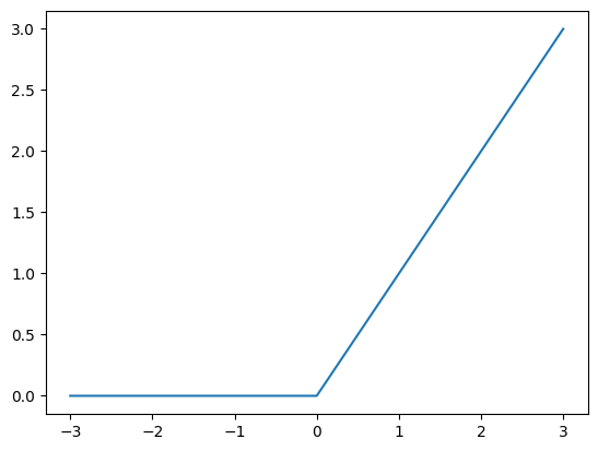
max and min of Two Functions

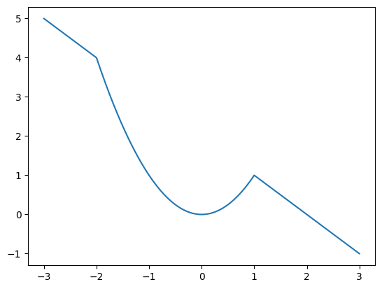
GFuncPy supports pointwise maximum and minimum operations using max and min. Here we plot the ReLU function and \(\min(x^2, 2-x)\).

from gfuncpy import Identity, max, min

x = Identity([-3, 3])

relu = max(x, 0)
relu.plot()

min(x**2, 2-x).plot()

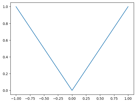
Making Your Functions Work with GridFunction

The @gfunc decorator lets you write custom univariate functions that work seamlessly with both scalars and grid-based data. When you pass a GridFunction, your decorated function is applied pointwise to every value on the grid, returning a new GridFunction; with a scalar, it behaves as the undecorated version.

from gfuncpy import gfunc, Identity

@gfunc
def absolute_value(x):
    if x > 0:
        return x
    else:
        return -x

x = Identity([-1, 1])

absolute_value(x).plot()

Performance Consideration

GFuncPy also supports NumPy’s built-in functions (like sin, cos, abs, etc.) directly on GridFunction objects—these are fast and vectorized, and should be preferred for most use cases. Use built-in NumPy functions and arithmetic for best performance, and @gfunc only when custom logic is needed. Like the above example can and should be done with NumPy’s built-in abs.

from gfuncpy import abs

abs(x).plot()